This article explores the principles and mechanisms behind the many popular Automatic Market Maker designs currently used in production. While the mathematical details of these designs are fascinating in their own right, this article seeks to instead focus on graphical representations and high-level concepts, allowing for a more approachable and exhaustive exploration of the space.

Watch our related Devcon 2022 talk here: https://www.youtube.com/watch?v=KxuyHfmLHP0.

Introduction

Historically, order books run by professional market makers have been the dominant method used to facilitate exchange. On-chain, maintaining an order book using traditional market-making tactics is prohibitively expensive, since storage and computation on distributed ledgers are in short supply and high demand. For this reason, Automatic Market Makers (AMM) have emerged as an efficient class of methods to facilitate the exchange of crypto assets on distributed ledgers. An AMM leverages smart contracts to allow permissionless participation in market-making by individuals seeking yield. These individuals passively provide liquidity to the contract, which can then use a predetermined function to automatically facilitate exchanges between buyers and sellers. The design of this procedure involves many tradeoffs that ultimately affect the utility of the platform to both liquidity providers and traders.

To understand AMM design tradeoffs, we must first understand that the ultimate goal of a market maker (both traditional and automatic) is to generate yield on a portfolio of assets by providing liquidity for trades in a market [1]. Yield will be the net result of fee/spread revenue earned on trading volume minus the change in the value of the portfolio. In AMMs this portfolio value change manifests as a so-called “impermanent loss”, since the portfolio value will decrease as the price deviates from the initial price, but will revert if the price moves back towards the initial one. Oftentimes this concept of a portfolio losing value as price moves is framed as a unique problem with AMMs, but this is only because AMMs allow it to be described and analyzed mathematically. Generally, losing portfolio value as the price moves is always a problem with market making, since by definition as a market maker you are allowing traders to exchange the less desirable asset for the more desirable asset. In this way, you will naturally receive more of the asset that is decreasing in value, and less of the one that is increasing. The market maker turns a profit when the revenue from spreads and/or fees outweighs this portfolio value change.

In AMMs this spread/fee revenue is typically collected by applying a near-one multiplier on the input or output of each trade. For instance, if an AMM wanted to charge a 0.3% fee, it could multiply the input by 0.997 and keep 0.003 * input as revenue for its liquidity providers. Setting this value can have a large impact on liquidity provider returns, and a tradeoff must be found between profiting as much as possible from each trade (higher fees) and maximizing the number of trades (lower fees). The optimal value will typically depend on the type of assets in the portfolio, as well as the type of AMM being used (the subject of the rest of the article). For more stable assets where portfolio risk is lower, lower fees are typically optimal, while more volatile assets typically demand higher fees to compensate for the risk. Many AMM implementations will add additional logic for dynamic fees, which can increase or decrease depending on fluctuating risk factors (e.g. price volatility can lead to inaccurate pricing).

Basic Automatic Market Makers

The first and most well-known AMM is the Constant Product Market Maker (CPMM), first released by Bancor in the form of bonding curves within “smart token” contracts, and then further popularized by Uniswap as an invariant function [2][3]. The CPMM spreads liquidity out equally between all prices, automatically adjusting the price in the direction of each trade made. This makes it an extremely general solution, allowing CPMMs to facilitate exchange between any arbitrary pair of assets. This generality though also turns out to be the primary weakness of CPMMs: providing equal liquidity at all exchange rates means that only a small portion of the liquidity can be provided at the current exchange rate. A better intuition for these mechanics can be achieved by walking through a few trade examples, as is done here [4]. This means that a CPMM can only facilitate trade sizes that are a small fraction of its total value locked (TVL) before experiencing significant price impact, making them very capital inefficient. Thus, while the CPMM has proven itself an essential member of the AMM ecosystem (especially for long-tail assets), there have been a wide range of AMMs created since the CPMM’s inception that seek to improve upon this design.

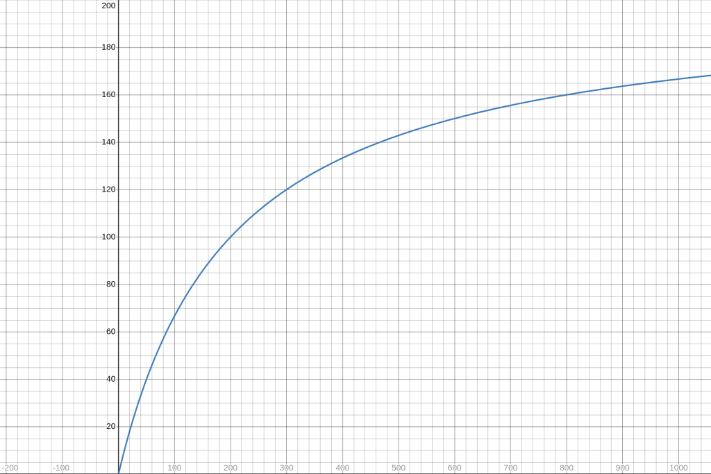
One such design is the Constant Mean Market Maker (CMMM), first introduced by Balancer Protocol [5]. The CMMM generalizes the CPMM by allowing the liquidity provider to specify desired portfolio weights, such as a 20%-80% split. In comparison, the CPMM lacks this customization and therefore always enforces an equal 50%-50% portfolio split. This generalization provides more flexibility to liquidity providers to adjust their market-making portfolios, but the underlying design and results are still the same as the CMMM discussed above. For the sake of simplicity, the rest of the article will typically refer to the CPMM, but will generally also apply to the CMMM.

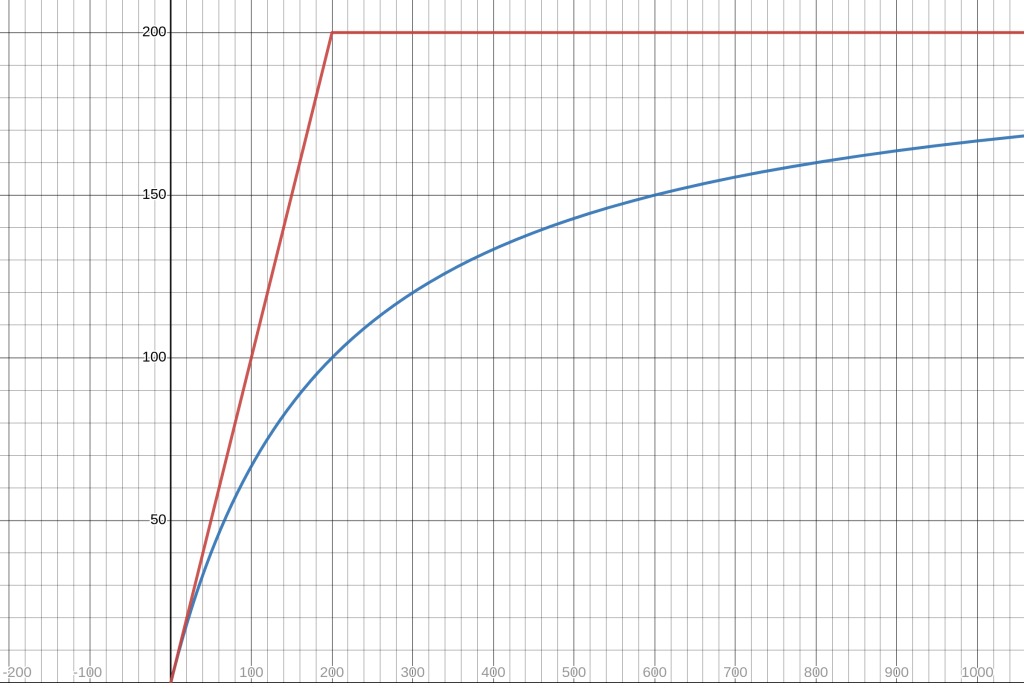
To outperform the CPMM, some prior assumptions about the market exchange rate of the assets must be made. This is not without risks, since making the wrong assumption can cause the market maker to exchange a large portion of its portfolio at the incorrect rate, causing the change in portfolio value to outweigh any fees collected. The extreme case of this is a Constant Sum Market Maker (CSMM), which facilitates exchange at a fixed rate regardless of the current portfolio the market maker holds. This allows for perfect capital efficiency at the selected exchange rate, but also quickly leads to the market maker losing all of the more valuable assets the moment the price deviates from the preselected value (at which point the portfolio is worth significantly less, and can no longer facilitate trades). For those familiar with Bayes theorem, many parallels can be seen here [6]. Using an outside oracle price (such as a 1:1 exchange rate for stablecoins) can be seen as using a prior, while adjusting the price in response to swaps (changes to your portfolio) can be seen as the likelihood. Under this lens, the CPMM can be seen as only using the likelihood with an infinitely diffuse prior, while a CSMM can be seen as utilizing only the prior and ignoring the likelihood. In the absence of any reasonable prior/oracle price (as is often the case in DeFi), the CPMM is a great choice. The CSMM only makes sense if you have complete trust in your prior/oracle price, which is rarely a good idea. Thus, the best option is usually a mixture of the two, which is what the bulk of AMM research focuses on.

Hybrid Automatic Market Makers

For the reasons stated above, CSMMs are rarely used in practice. In theory, they sound great for facilitating trades between assets that should theoretically have the same value, such as two stablecoins. But, in practice, small fluctuations in desirability between these assets will still leave the market maker with only the less desirable asset (not to mention the risk of one de-pegging completely). This was some of the motivation behind Curve introducing a more efficient solution to this problem called StableSwap, our first example of a hybrid AMM [7]. Like a CPMM, a StableSwap market maker will adjust its exchange rate as its portfolio changes, but, unlike a CPMM (and like a CSMM), it will do so very slowly at first, maintaining close to a 1:1 exchange rate for longer. As the price deviates farther and farther from the 1:1 exchange rate, the rate at which the price is adjusted accelerates, such that the market maker is never left holding only one asset. The rate at which this process accelerates is adjustable via an amplification coefficient parameter set for each pool. This model has become the industry standard for assets pegged to the same external asset but has not seen much use outside of this specific use case.

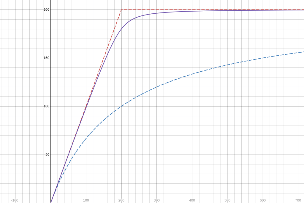
An alternative algorithm for swapping stable assets was more recently introduced by Solidly, which builds on Uniswap V2 by adding an option to create a pair specialized for stable assets [8]. Unlike a normal Uniswap V2 pair, this pair utilizes a quartic sum invariant instead of the usual quadratic invariant (but retains the same interface). This flattens the curve around the 1:1 exchange rate and produces a very similar effect to StableSwap, but lacks an adjustment parameter similar to the amplification coefficient mentioned above. Empirically, the curve seems to provide similar output to StableSwap with an amplification coefficient of 2 (see below figure), which is much lower than is typically used in StableSwap pools. This makes it a bit lower risk (without additional tuning) for a wider range of stable assets that may have larger fluctuations around their peg, but it also may be slightly less efficient for those that do not.

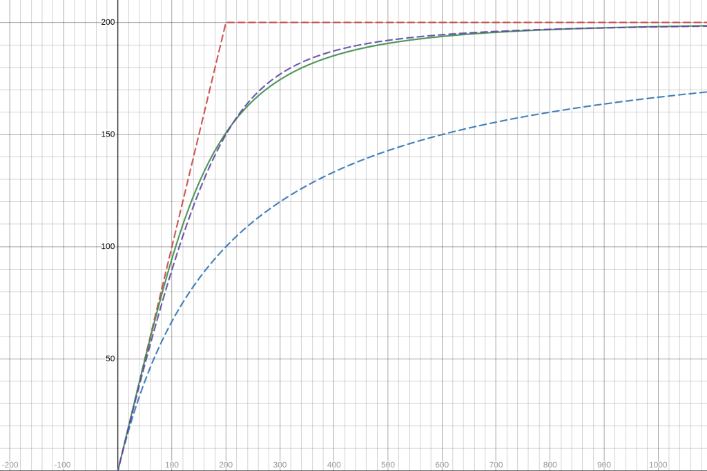
Other AMMs similarly aim to interpolate between a constant sum and constant product model, but also expand their scope beyond pegged assets. Dodo develops a Proactive Market Maker (PMM) algorithm that aims to flatten the price curve around an oracle price [9]. This oracle price can be set to 1 for pegged asset pairs, but can also utilize Chainlink oracles for volatile pairs. At a high level, the PMM algorithm aims to maintain target reserve values (how much of each asset it would like to have) and gives decreasing rates the farther away the real reserves deviate from these values. The PMM exposes a slippage parameter, k, that allows the algorithm to interpolate between a constant product market maker (k = 1) and a constant sum/fixed rate market maker (k = 0). The math for calculating trades with this setup gets a bit messy, requiring integration under some scenarios, and solving for quadratic roots under others. Regardless, it has proven itself to be an effective mechanism to provide capital-efficient liquidity.

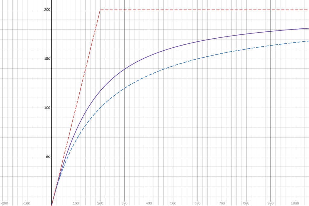
Clipper develops an AMM that has a similar result but gets there in a very different way [10]. Clipper more explicitly derives a solution that interpolates between constant sum and constant product by combining the constant sum model, wherein assets are exchanged at a fixed price, and a constant product model, where assets are exchanged according to the ratio of reserves held by the market maker. Similar to Dodo, these two extremes are combined on a continuous spectrum parameterized by a slippage parameter, k. The resulting interpolation is a bit different, however — the most concrete difference is that, unlike Dodo, a clipper AMM is actually capable of giving away all of one asset (like a constant sum market maker). This can become particularly dangerous for configurations closer to a CSMM (k close to 0) with an unreliable oracle.

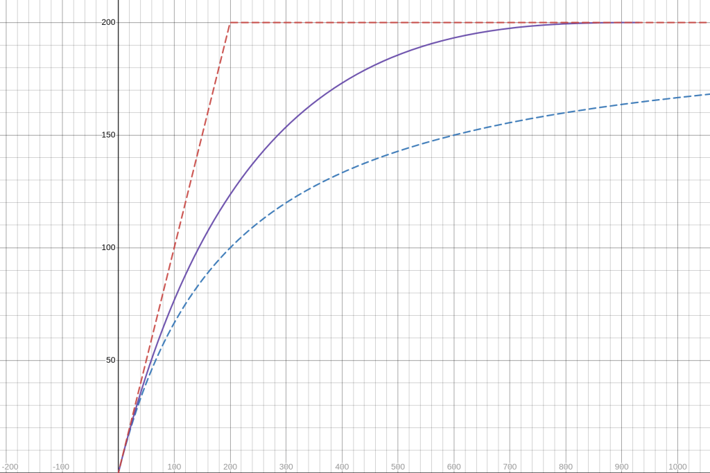
Curve, the originator of StableSwap, has also released a new AMM for volatile assets called CryptoSwap [11]. CryptoSwap expands on the StableSwap algorithm by adding another parameter enabling quicker switching into price discovery mode (constant product) as the price moves away from the peg. This makes the algorithm better at handling a dynamic peg, allowing it to be used for more volatile assets. Curve’s CryptoSwap implementations also include a dynamic fee and an internal oracle system, making it unique in that respect since most other solutions use fixed rates or Chainlink oracles [12]. Implementing this AMM requires solving cubic, sextic, and higher-degree equations, which is typically done in practice using Newton’s Method [13]. This combined with its internal oracle and dynamic fees makes it one of the most complex AMMs currently in use. (For this reason, a CryptoSwap graph is omitted.) It is still early in its life cycle, so it remains to be seen whether this extra complexity translates into a better-performing AMM. So far it has mostly seen its use limited to one pool filled with the highest market cap assets on a given chain. Recently, though, it has been getting rolled out in more pools, growing its reach in the AMM space.

Virtual Reserve Automatic Market Makers

An alternative way to achieve greater capital efficiency is to use virtual reserves, a concept first introduced by KyberSwap [14]. Virtual reserve AMMs utilize the CPMM model but multiply the real balances of each asset by an amplification factor. The result is that a much higher capital efficiency can be provided over the CPMM (bringing in more volume and fee revenue), but the market maker loses the CPMM’s ability to never run out of either asset. In this way, the amplification factor allows a tradeoff between capital efficiency and extra portfolio risk. Generally, a high amplification factor can work well for stable pairs but becomes riskier the more volatile a pair gets.

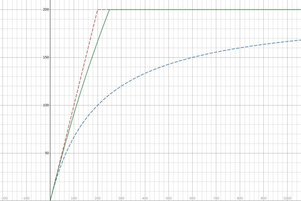
Uniswap V3 puts a very interesting spin on the concept of virtual reserves [15]. Instead of imposing one constant amplification coefficient on the entire pool, Uniswap V3 allows each liquidity provider to pick their own price range (and implicitly their own amplification parameter to span that range). Liquidity providers take on more portfolio risk with tighter price range positions (implicitly this means higher amplification coefficients), but also accrue proportionally more fees for trades within this range. In this way, Uniswap V3 can be seen as using incentives (higher yield for picking the true price range as precisely as possible) to source the best tradeoff in capital efficiency and portfolio risk at a given point, even for two volatile assets. This model has proven extremely effective, but also generally requires liquidity providers to be more active and informed in order to receive a good yield. Naive liquidity provision over the entire price range will typically result in a much lower fee share, while aggressive but mismanaged liquidity provision will typically lead to portfolio value loss outweighing any fee revenue. The development of intelligent automated liquidity managing strategies will likely continue to make these (and similar) AMMs more effective, and the corresponding yield opportunities more competitive.

Request For Quote Systems

As a footnote, it is worth mentioning Request For Quote (RFQ) systems. RFQ mechanisms allow for private off-chain pricing with on-chain settlement and portfolio custody, allowing the gap between DeFi and traditional finance to be bridged. To utilize such a system, a centralized API must be queried for a quote, which can then be used on-chain to execute the trade. Off-chain pricing has the advantage of allowing for the use of off-chain information. This can include any of a range of private market-making tactics, including a marginal rate structure (used by Hashflow), or more traditional order book methods used by centralized exchanges [16]. Alternatively, high-frequency tuning of AMM equations can be done to achieve better performance than their on-chain counterparts. One example of this is Clipper’s Formula Market Maker (FMM). Clipper’s FMM uses a rapidly updating live price feed as the oracle price in their AMM formula (discussed above), allowing them to shift closer to a CSMM and achieve greater capital efficiency [17].

Conclusions

While the above list of AMMs gives an overview of the space and covers many of the major DEXs that currently hold a high TVL, there remain several significant AMMs that were not covered (not to mention the many more currently being built). Recently, a new class of DeFi projects has even started designing paradigms that aim to generalize to any curve. Primitive Finance makes use of a Replicating Market Maker (RMM), which is able to construct an AMM curve from any of a large range of possible liquidity provider payoffs [18]. Shell protocol recently introduced a new AMM called Proteus — it is constructed from conic sections and contains 6 parameters, giving it the ability to be fit to a very wide range of desired curves [19]. While out of the scope of this article, there is also an ever-growing selection of protocols that offer financial derivatives, such as options and perpetuals.

With the enormous variation in AMM models and fragmentation in the liquidity used to facilitate trades, DEX aggregators have become an essential part of the DeFi ecosystem. DEX aggregators collect information about all liquidity sources on a given chain (including all AMM models discussed above) and then attempt to find the best combination of actions in order to get the best rate for a given trade. Oftentimes, the optimal route can contain many hops and complex splitting, making it an extremely hard problem to solve. Odos.xyz is a new DEX aggregator that is able to search more complex solutions than existing platforms, allowing for atomic multi-input trades and better rates for its users.

[1] https://www.investopedia.com/terms/m/marketmaker.asp
[2] https://cryptorating.eu/whitepapers/Bancor/bancor_protocol_whitepaper_en.pdf
[3] https://uniswap.org/whitepaper.pdf
[4] https://jfin-swufe.springeropen.com/articles/10.1186/s40854-021-00314-5#Sec5
[5] https://balancer.fi/whitepaper.pdf
[6] https://en.wikipedia.org/wiki/Bayes%27_theorem
[7] https://curve.fi/files/stableswap-paper.pdf
[8] https://pontem.network/posts/everything-you-need-to-know-about-solidly-the-latest-project-by-andre-cronje
[9] https://docs.dodoex.io/english/dodo-academy/pmm-overview/the-mathematical-principle-of-pmm
[10] https://github.com/shipyard-software/market-making-whitepaper
[11] https://classic.curve.fi/files/crypto-pools-paper.pdf
[12] https://research.chain.link/whitepaper-v2.pdf
[13] https://en.wikipedia.org/wiki/Newton%27s_method
[14] https://files.kyber.network/DMM-Feb21.pdf
[15] https://uniswap.org/whitepaper-v3.pdf
[16] https://docs.hashflow.com/hashflow/
[17] https://www.shipyardsoftware.org/post/what-is-a-fmm
[18] https://stanford.edu/~guillean/papers/rmms.pdf
[19] https://shellprotocol.io/static/Proteus_AMM_Engine_-_Shell_v2_Part_1.pdf