Indexer Allocation Optimization: Part II

This article was co-authored with Howard Heaton, from Edge & Node, and with Hope Yen, from GraphOps.

TL;DR

Analytically optimizing to maximize indexing rewards may seem like a straightforward solution, but it oversimplifies the complexities involved in an indexer’s decision-making process. In this post, we’ll discuss how we enable indexers to input their preferences into the Allocation Optimizer and how those preferences can impact the Allocation Optimization problem. We’ll also explore how we incorporate a gas fee to make the optimization problem more realistic, which results in a non-convex problem.

Overview

In Part I, we provided an overview of the Indexer Allocation Optimization problem and discussed how we can optimize for a basic version of it. However, indexers have unique preferences and constraints that cannot be easily represented in the math model. Additionally, we need to factor in gas costs, which are a per-allocation fee that indexers incur when they allocate. In this section, we’ll address both indexer preferences and gas costs, one at a time. It’s important to note that while we will use some math concepts, we’ll strive to explain them in a way that’s accessible to readers with a college undergraduate level of math knowledge, by which we mean a basic knowledge of calculus and linear algebra.

Optimizing Over Gas

Gas costs have long been a challenging issue for those seeking to solve web3 optimization problems, with a variety of proposed solutions. For instance, Angeris et al.’s paper on optimal routing for constant function market makers[1] proposes one approach using convex relaxation. In this section, we’ll offer our own take by framing the problem of optimal allocation with fixed transaction costs as a sparse vector optimization problem. Specifically, we aim to find the set of optimal sparse vectors and then select the specific sparse vector that yields the highest profit. We define profit as the total indexing reward minus the total gas cost. In the following section, we’ll go through the background math at a very high level. For the most part, we use images to make our points. However, if you’d rather not understand how the algorithm works, feel free to skip over it and jump to the section “Indexer Profits.”

The Math At A Glance

Let’s take a look at an example. Say we want to minimize the function

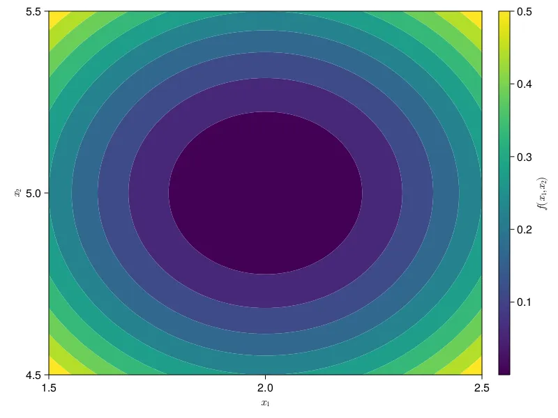
\begin{equation} f(x_1, x_2) = (x_1 - 2)^2 + (x_2 - 5)^2 \end{equation}

Convex contour plot — A filled contour plot of Eq. 1.

You should hopefully be able to see that this happens at $(2, 5)$ . Plug those numbers in for $x_1$ and $x_2$ if you can’t. The result should be $0$ . This is obvious to see, but let’s see if we can do this in a more automated way.

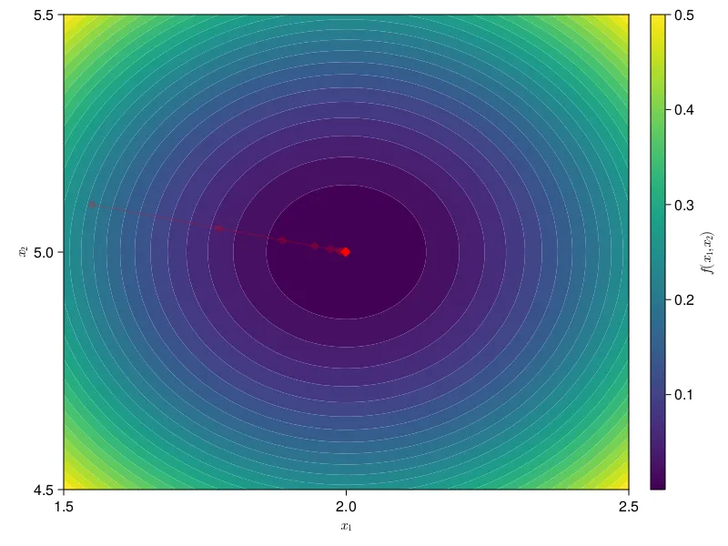
One way to do this is gradient descent. Here’s how it works. Pick some random point $x^{(1)}$ to start the algorithm from. The gradient of the function $\nabla f$ gives you the direction of steepest ascent. Since we want to find the minimum, we put a negative sign in front of it. We step in the direction of the negative gradient with step size $\eta$ . Thus, our update rule becomes.

\begin{equation} x^{(n+1)} = x^{(n)} - \eta \nabla f(x^{(n)}) \end{equation}

Note: If you aren’t interested in the math, feel free to skip ahead to the paragraph above the next image.

Let’s plug in our $f$ and see this in action.

\begin{equation*} f(x_1, x_2) = (x_1 - 2)^2 + (x_2 - 5)^2 \end{equation*}

We’ll split this into two parts - solving for $x_1$ and solving for $x_2$ independently. Let’s start with $x_1$ . First, we find the gradient of $f$ with respect to $x_1$ .

\begin{equation*} \frac{\partial f}{\partial x_1} = 2(x_1 - 2) = 2x_1 - 4 \end{equation*}

Now, we use the formula for gradient descent and start plugging in numbers.

\begin{align*} x^{(n+1)}_1 &= x^{(n)}_1 - \eta \frac{\partial f}{\partial x_1} \\ &= x^{(n)}_1 - \eta (2x^{(n)}_1 - 4) \\ &= x^{(n)}_1 -2\eta x^{(n)}_1 + 4\eta \\ &= (1 - 2\eta)x^{(n)}_1 + 4\eta \end{align*}

We can now replace $x^{(n)}$ with the same gradient descent formula applied to $x^{(n-1)}$ .

\begin{align*} x^{(n+1)}_1 &= (1 - 2\eta)\left[(1-2\eta)x^{(n-1)} + 4\eta\right] + 4\eta \\ &= (1 - 2\eta)^2x^{(n-1)}_1 + \left[(1 - 2\eta)4\eta + 4\eta\right] \end{align*}

I grouped certain terms together on purpose. Hopefully, you can sort of see the pattern at this point. If not, I recommend you do the math again. Regardless, if we want to write $x^{(n+1)}$ in terms of $x^{(n-2)}$ , we can do this as

\begin{equation*} x^{(n+1)}_1 = (1 - 2\eta)^2x^{(n-2)}_1 + \left[(1 - 2\eta)^24\eta + (1 - 2\eta)4\eta + 4\eta\right] \end{equation*}

And if we keep doing this, we get

\begin{equation*} x^{(n+1)}_1 = (1 - 2\eta)^nx^{(1)}_1 + \left[(1 - 2\eta)^{n-1} + (1 - 2\eta)^{n-2} + ... + 1\right]4\eta \end{equation*}

You should hopefully recognize the term in the square brackets as a geometric series. If $|\eta| < 1$ , this converges to give us

\begin{equation*} x^{(n+1)}_1 = (1 - 2\eta)^nx^{(1)}_1 + \frac{1 - (1 - 2\eta)^n}{1 - (1 - 2\eta)}4\eta \end{equation*}

Notice here that we must have $|1 - 2\eta| < 1$ . Else, the $(1 - 2\eta)^n$ terms blow up to infinity. If we select $\eta$ to be such that that inequality is satisfied, notice that every $(1 - 2\eta)^n$ goes to $0$ as $n \to \infty$ . Thus, as $n \to \infty$ , we can rewrite our formula as

\begin{equation*} x^{(n+1)}_1 = \frac{1}{2\eta}4\eta = 2 \end{equation*}

Thus, our optimal $x_1 = 2$ . Notice this is exactly what we’d found visually earlier. The only difference is that now we’ve used a less manual algorithm instead. If our function $f$ satisfies certain properties, we are guaranteed to find the global minimum using gradient descent. The full list of properties is beyond the scope of this post. We’ll just focus on one - convexity.

Convex gradient descent — Gradient descent on Eq. 1. The red line shows the trajectory the algorithm takes to reach the optimal value. The bright red diamond is the optimal value.

A convex function $f$ is a function that always curves upwards. This means that for two points in $a$ and $b$ , the line segment connecting $f(a)$ to $f(b)$ is always on or above the curve of $f$ . So $x^2$ is convex; $x^3$ is not. $-x^2$ is concave, which is fine because we can just run gradient ascent to find the maximum instead of gradient descent to find the minimum. We’ll come back to convexity a bit later.

Now, that we know we can use gradient descent to minimize an objective function, let’s be a bit more interesting. Let’s say there are constraints on our solution. Let’s say that I have a maximum of 10 units I can divide between $x_1$ and $x_2$ . This is totally fine, because 2+5=7 which is less than 10. Now let’s say instead that I have just 1 unit I can allocate. Would I be better off dividing this between $x_1$ and $x_2$ , or would it be better to go all in on one? This is no longer as obvious.

In Part I, we talked about using the Karush-Kuhn-Tucker conditions to solve this problem, and this is what gave us our analytic solution. Now, we want to continue on this theme of finding a more general solution. In this case, we can use projections.

This new constraint, that the $x_1 + x_2 = 1$ and that $x_1 \geq 0$ and $x_2 \geq 0$ , has a name - the simplex constraint. The simplex constraint has a corresponding simplex projection.[2] We’ll use this here. I won’t talk through the math again. If you’re interested, feel free to work it out for yourself. I’ll just give you the new update rule.

\begin{equation} x^{(n+1)}_1 = T(x^{(n)} - \eta \nabla f(x^{(n)})) \end{equation}

In other words, we take our normal gradient descent step, and then we project the result of that onto the simplex, which is denoted by the operator $T$ . What does this look like?

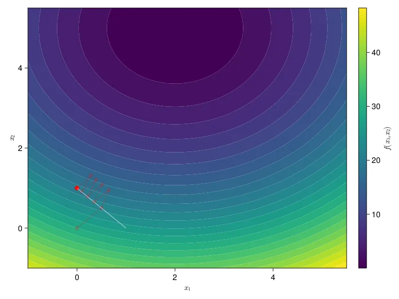
Projected gradient descent onto the unit-simplex for Eq. 1. The white line denotes the feasible region.

We revisit our familiar problem $f(x_1, x_2) = (x_1 - 2)^2 + (x_2 - 5)^2$ . Now we add a unit-simplex constraint ( $x_1 + x_2 = 1$ ; $x_1 \geq 0$ , $x_2 \geq 0$ ). In the above figure, we set $x^{(1)} = (0, 0)$ . From here, we first project this onto the unit simplex. The white line shows the feasible region of the unit-simplex constraint, meaning all the possible combinations of $(x_1, x_2)$ that satisfy the expressions from before. The projection operation $T(x)$ simply finds the closest $x'$ that is in the feasible region (on the white line). You can see this happening in our plot. First $x^{(1)} = (0, 0)$ gets projected onto $(0.5, 0.5)$ . Then, we take a step of gradient descent, pulling us off the feasible region in the direction of the true optimal, which we know from before to be $(2, 5)$ . Then our projection brings us back onto the feasible region. We repeat this until we converge to the optimal value for our new problem $(0, 1)$ .

Let’s add another layer of complexity again. Let’s say we know for a fact that our solution is sparse - meaning the solution is either $(0, 1)$ or $(1, 0)$ . Can we do any better than this back-and-forth stepping? We treat this as a new constraint, which we call a sparsity constraint - the number of nonzero elements of $x$ should be at most $k$ . In this case, $k = 1$ . Sparse projections onto the simplex are again a common type of problem, so we’ll refer you to the cited paper if you want to learn more.[3] In any case, we can now use the Greedy Selector and Simplex Projector (GSSP) algorithm in place of where we’d used the simplex projection before.

Using GSSP converges a lot quicker, but actually gets stuck on the wrong point. It gets stuck on $(1, 0)$ rather than $(0, 1)$ . We can check that this is a worse solution by plugging both of those points back into our objective function. $f(1, 0) = 26$ and $f(0, 1) = 20$ . Since we’re minimizing, the latter is better. Is there anything we can do here?

Of course! We know the optimal unconstrained point. We were even able to just look at the plot and see that it is $(2, 5)$ . We’ll use this an an anchor point in Halpern iteration.[4] Again we won’t go through the mathematical details of the algorithm other than to point you to the paper. Instead, we’ll just talk through the algorithm visually.

At a high level, Halpern iteration will try to anchor our solution to some anchor point $x_a = (2, 5)$ . What this means is that we’ll first pull the solution towards $(2, 5)$ , and then use GSSP to project the solution back onto the simplex. As the number of iterations increases, the pull of the anchor point lessens to the point at which it drops off completely, and we’re left with just the vanilla projected gradient descent with GSSP that we talked about before. This is equivalent to adding a new operator $H$ that executes Halpern iteration during our projected gradient descent update.

\begin{equation} x^{(n+1)}_1 = T(H(x^{(n)} - \eta \nabla f(x^{(n)}))) \end{equation}

Indexer Profits

Back to our problem. Instead of our dummy $f(x)$ , now we use the indexing reward.

\begin{align*} \min_{\Omega_i} \quad & -\sum_{j \in \mathcal{S}}\frac{\Omega_{ij}}{\sum_{k \in \mathcal{I}} \Omega_{kj}}\cdot\Phi\frac{\psi_j}{\sum_{l \in \mathcal{S}} \psi_l} \\ \textrm{s.t.} \quad & \omega_k \geq 0 \quad \forall \ \omega_k\in\Omega_i \\ \quad & \sum_{j\in\mathcal{S}}\Omega_{ij} = \sigma_i \end{align*}

If this notation is unfamiliar, please refer back to Part I. We will call the above formulation A. Notice our constraints are actually a simplex constraint - they take the form $\sum_i x_i = C$ , $x_i \geq 0 \ \forall i$ . This means we can solve this problem using the simplex projection we talked about in the previous section. Use gradient descent to step in the direction of an optimum; then, use the simplex projection to bring ourselves back onto the feasible region. As in the last section, we can use the optimal value computed analytically, as shown in Part I as our anchor for Halpern iteration. This is, in fact, what the Allocation Optimizer does. Well, almost.

So far, we’ve talked about indexing rewards. We are actually concerned with indexer profits. Our optimization problem is now

l \begin{align*} \min_{\Omega_i} \quad & -\sum_{j \in \mathcal{S}}\frac{\Omega_{ij}}{\sum_{k \in \mathcal{I}} \Omega_{kj}}\cdot\Phi\frac{\psi_j}{\sum_{l \in \mathcal{S}} \psi_l}+ 2g\sum_{j\in\mathcal{S}}\eta_j \\ \textrm{s.t.} \quad & \omega_k \geq 0 \quad \forall \ \omega_k\in\Omega_i \\ \quad & \sum_{j\in\mathcal{S}}\Omega_{ij} = \sigma_i \end{align*}

We’ll call this formulation B.

B is a problem. Our objective function, which was convex in A, is no longer so. This is because we’ve added a new term depending on $\eta_j$ , which is a binary variable such that it has value $\eta_j = 1$ if $\omega_j > 0$ and 0 otherwise. This is a big problem for us. Too see why, consider the picture below.

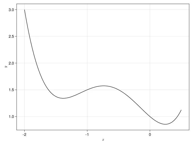
The plot above shows a non-convex function. Consider the problem of using gradient descent to minimize it. As a reminder, gradient descent follows the slope down. Once the slope shifts from negative to positive, gradient descent is done. In the above plot, we have two minima, one that is at $x>0$ and one that is at $x<0$ . Let’s imagine we start gradient descent from $x>1$ . What happens? Well, gradient descent will slide leftwards until it reaches the rightmost minimum. Now imagine, that we start from $x<-2$ . What happens now? Gradient descent will step rightwards until it hits the leftmost minimum. Except this isn’t the best we could have done. We actually could have gone further and found a better solution. Here’s the problem we now face put more directly. We can use gradient descent just fine on non-convex functions, but how do we know we’ve actually reached the global minimum, rather than a local minimum? How do we know we couldn’t do better than the solution we found? As I’ve mentioned before, this style of problem, in which a convex function becomes non-convex due to gas fees, is everywhere in web3. Let’s talk about one of the potential solutions to this.

For the sake of argument, let’s pretend there were 10 subgraphs on the network. If an indexer wanted to allocate, they could allocate on one subgraph, or two subgraphs, or three subgraphs, all the way up to ten subgraphs. Each subsequent allocation vector (from 1 nonzero to 10) would have increasing gas costs corresponding with the $\eta_j$ term in B. What we could do is solve A with an additional sparsity constraint.

\begin{align*} \min_{\Omega_i} \quad & -\sum_{j \in \mathcal{S}}\frac{\Omega_{ij}}{\sum_{k \in \mathcal{I}} \Omega_{kj}}\cdot\Phi\frac{\psi_j}{\sum_{l \in \mathcal{S}} \psi_l} \\ \textrm{s.t.} \quad & \omega_k \geq 0 \quad \forall \ \omega_k\in\Omega_i \\ \quad & \sum_{j\in\mathcal{S}}\Omega_{ij} = \sigma_i \\ \quad & \sum_{j\in\mathcal{S}}\eta_j \leq k \end{align*}

We’ll call this formulation C. If we solve C for each value $k$ from 1 to the number of subgraphs, then we’ll have our optimal allocation strategy if the indexer opens one new allocation, the optimal strategy for two allocations, and so on. Then, we can choose the best of these by picking the one that minimizes the objective function of B. We already know how to solve problems with a sparse simplex constraint. Just use GSSP!

When you run the Allocation Optimizer with opt_mode = "fast", this is exactly what the code does! In summary, solve C using projected gradient descent with GSSP and Halpern iteration. Then, for each of these possible allocation vectors, compute the magnitude of the objective function of B. Finally, return the allocation strategy with the lowest magnitude.

Results

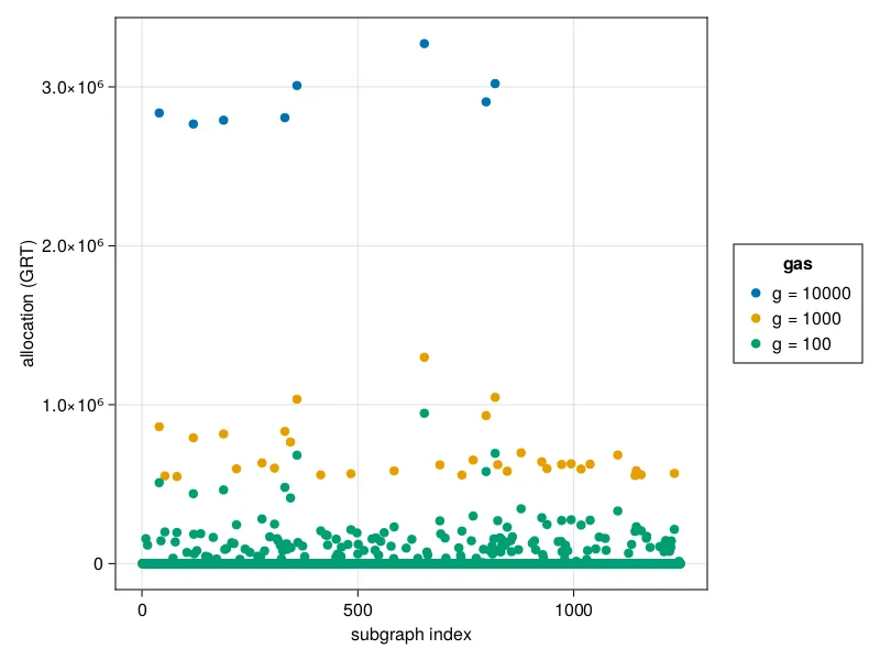
	100 GRT	1000 GRT	10000 GRT
Current Profit	191525.88	183425.88	102425.88
Optimized Profit	540841.27	469017.12	333127.37
% Increase	282%	255%	325%

Comparing the indexer’s current allocation strategy to the optimized allocation strategies from the table. For example, the indexer’s profit at a gas cost of 100 GRT is compared with the green strategy in the plot.

If you recall from Part I, we were originally concerned that the analytic solution allocated to way more subgraphs than indexers did. This was in part due to the fact that the analytic solution does not respect gas costs. Here, we demonstrate that the new algorithm does so, and also manages to outperform the indexer’s existing allocation strategy across a variety of different gas costs. Other than gas costs, the Allocation Optimizer also enables indexers to further pare down this via other entries in the configuration file. Let’s run through those.

Indexer Preferences

There is no way our optimizer could compensate for the full diversity of thought behind how different indexers choose to allocate. Some may prefer shorter allocations. Others may prefer to keep their allocation open for a maximum of 28 epochs (roughly 28 days). Some indexers may have strong negative or positive feelings towards specific subgraphs. In this section, we talk through how the Allocation Optimizer accounts for this information.

Filtering Subgraphs

Indexers often don’t care to index some subgraphs. Maybe a subgraph is broken. Maybe it’s massive, and the indexer just won’t be able to sync it in a short amount of time. Whatever the reason, we want to ensure that indexers have the ability to blacklist subgraphs. In the previous post, we used the notation $\mathcal{S}$ to represent the set of all subgraphs. To remove blacklisted subgraphs from the optimization problem, all we do is choose some set $\mathcal{S}' = \mathcal{S}\backslash \mathcal{B}$ where $\mathcal{B}$ is the set of blacklisted subgraphs.

Since indexing a subgraph takes time, many indexers also have a curated list of subgraphs that they already have synced or mostly synced. They may only want to allocate to subgraphs in that list. Therefore, indexers can also specify a whitelist in the configuration file. To see how the whitelist $\mathcal{W}$ modifies the math, all we have to do is replace all instances of $\mathcal{S}$ with $\mathcal{W}$ .

Let’s say an indexer is already allocated on a subgraph and does not want the Optimizer the try to unallocate from this subgraph. The indexer can specify this in the frozenlist. Subgraphs in the frozenlist are treated as though they are blacklisted. However, they differ from blacklisted subgraphs in that the indexer’s allocated stake on these frozen subgraphs $\sigma_f$ is not available for reallocation. Therefore, $\sigma' = \sigma - \sigma_f$ .

The final list we allow for is the pinnedlist. This is mostly meant to be used by so-called backstop indexers - indexers who are not necessarily there to make a profit from the network, but more just to ensure that all data is served. Pinned subgraphs are treated as whitelisted since the Optimizer may decide to allocate to them anyway. However, if the Optimizer doesn’t, we manually add 0.1 GRT back onto each of these subgraphs just so that the indexer has a small, non-negative allocation on the pinned subgraphs.

Beyond the lists, indexers may also choose to not be interested in subgraphs with signal less than some amount, even if it is optimal to be on said subgraph. Thus, they can specify a min_signal value in the configuration file. The Optimizer will filter out any subgraphs with signal below this amount.

Other Preferences

As we mentioned before, indexers may also choose to allocate for a variety of different time periods. Thus, they can specify the allocation_lifetime in the configuration file. This determined how many new GRT are minted from token issuance during that time frame, which is given by the classic $P(r^t - 1)$ where $P$ is the current number of GRT in circulation, $r$ is the issuance rate, and. $t$ is the allocation lifetime in blocks. As $t$ decreases, fewer tokens are issued, which means the effect of the gas term in our objective function becomes stronger.

The final preference that indexers can specify is max_allocations. For whatever reason, an indexer may prefer to allocate to fewer than the optimal number of subgraphs. Maybe this is due to hardware constraints on their side, or else perhaps it’s because of reduced mental load in tracking subgraphs. In any case, once indexers specify this number, the Optimizer uses it as $k_{max}$ . In other words, when it solves formulation C, normally it would solve it for $k \in [1,...,\textrm{number of subgraphs}]$ . Instead, it will solve it $k \in [1,...,k_{max}]$ times.

Conclusion

In Part II of the Allocation Optimizer series, we’ve demonstrated how the Allocation Optimizer accounts for indexer preferences and how the Val(:fast) mode solves the non-convex optimization problem using GSSP and Halpern iteration. We also demonstrated some results for the algorithm, showing that it outperforms a current indexer’s existing allocations. However, we did not demonstrate optimality. Spoiler alert, the Allocation Optimizer also has a Val(:optimal) flag. The solution we talked about here is fast, and will often outperform manually choosing allocations. However, we can do better. We’ll leave the details to our next blog post though.

Just a final note, if you’re interested in playing around with the techniques described in our blog post - gradient descent, projected gradient descent, the simplex projection, GSSP, and Halpern iteration, check out our Julia package SemioticOpt. The Allocation Optimizer and the code that generated the plots in this blogpost both use SemioticOpt.